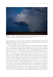
2 – Water – where, when, how much? 23 Australia) than the same volume and rate of extraction from a pathway which predominantly supplied the floodplain, where the impact would be predominantly on the ecosystem and landholders, depending on the floodplain. A second example of spatial variability is in South Australia, where the Cooper changes from an anastomosing channel system to a distributary channel system. Here, the Cooper splits into three distinct flow paths: Strzelecki Creek (only receiving flow from Cooper Creek during very large floods), the Main Branch (with two subsequent branches) and the North- west Branch (Fig. 2.5). The latter flow path supplies the iconic, Ramsar-listed Coongie Lakes (Fig. 2.6). To estimate how changes in the flow regime would affect inflows to Coongie Lakes, we need to know the thresholds and how much water flows down each of the flow paths for the range of different events. During April 2012, the flood pulse from Queensland (see Fig. 2.7) had approximately an annual recurrence interval and the North-west Branch received 53% of the channel flow while the rest (47%) went down the two channels that form the Main Branch. However, a flow double this volume in 2011 pushed a higher percentage of flow down one of the Main Branch channels (see Fig. 2.5): 34% compared to 20% of the flow in 2012. Flood conditions prevented the other Main Branch channel and the North-west Branch channel from being measured in 2011. Clearly, the percentage of flows down the different channels varies with the volume of the flow, but this is difficult to determine even in a medium volume flood, requiring substantial effort to collect such critical data in this remote and challenging environment. Unless these changes in the percentages in Fig. 2.4. Local storms in the Lake Eyre Basin make a contribution to the flow of the rivers in the Lake Eyre Basin into waterholes, floodplains and lakes (photo, A. Emmott).